10 Minutes to Dask#
This is a short overview of Dask geared towards new users. There is much more information contained in the rest of the documentation.

High level collections are used to generate task graphs which can be executed by schedulers on a single machine or a cluster.#
We normally import Dask as follows:
>>> import numpy as np
>>> import pandas as pd

>>> import dask.dataframe as dd
>>> import dask.array as da
>>> import dask.bag as db
Based on the type of data you are working with, you might not need all of these.
Creating a Dask Object#
You can create a Dask object from scratch by supplying existing data and optionally including information about how the chunks should be structured.
See Dask DataFrame.
>>> index = pd.date_range("2021-09-01", periods=2400, freq="1h")
... df = pd.DataFrame({"a": np.arange(2400), "b": list("abcaddbe" * 300)}, index=index)
... ddf = dd.from_pandas(df, npartitions=10)
... ddf
Dask DataFrame Structure:
                        a       b
npartitions=10
2021-09-01 00:00:00  int64  object
2021-09-11 00:00:00    ...     ...
...                    ...     ...
2021-11-30 00:00:00    ...     ...
2021-12-09 23:00:00    ...     ...
Dask Name: from_pandas, 10 tasks
Now we have a Dask DataFrame with 2 columns and 2400 rows composed of 10 partitions where each partition has 240 rows. Each partition represents a piece of the data.
Here are some key properties of a DataFrame:
>>> # check the index values covered by each partition
... ddf.divisions
(Timestamp('2021-09-01 00:00:00', freq='H'),
Timestamp('2021-09-11 00:00:00', freq='H'),
Timestamp('2021-09-21 00:00:00', freq='H'),
Timestamp('2021-10-01 00:00:00', freq='H'),
Timestamp('2021-10-11 00:00:00', freq='H'),
Timestamp('2021-10-21 00:00:00', freq='H'),
Timestamp('2021-10-31 00:00:00', freq='H'),
Timestamp('2021-11-10 00:00:00', freq='H'),
Timestamp('2021-11-20 00:00:00', freq='H'),
Timestamp('2021-11-30 00:00:00', freq='H'),
Timestamp('2021-12-09 23:00:00', freq='H'))

>>> # access a particular partition
... ddf.partitions[1]
Dask DataFrame Structure:
                  a       b
npartitions=1
2021-09-11     int64  object
2021-09-21       ...     ...
Dask Name: blocks, 11 tasks
See Array.
import numpy as np
import dask.array as da

data = np.arange(100_000).reshape(200, 500)
a = da.from_array(data, chunks=(100, 100))
a
|
||||||||||||||||
Now we have a 2D array with the shape (200, 500) composed of 10 chunks where each chunk has the shape (100, 100). Each chunk represents a piece of the data.
Here are some key properties of a Dask Array:
# inspect the chunks
a.chunks
((100, 100), (100, 100, 100, 100, 100))
# access a particular block of data
a.blocks[1, 3]
|
||||||||||||||||
See Bag.
>>> b = db.from_sequence([1, 2, 3, 4, 5, 6, 2, 1], npartitions=2)
... b
dask.bag<from_sequence, npartitions=2>
Now we have a sequence with 8 items composed of 2 partitions where each partition has 4 items in it. Each partition represents a piece of the data.
Indexing#
Indexing Dask collections feels just like slicing NumPy arrays or pandas DataFrame.
>>> ddf.b
Dask Series Structure:
npartitions=10
2021-09-01 00:00:00    object
2021-09-11 00:00:00       ...
                        ...
2021-11-30 00:00:00       ...
2021-12-09 23:00:00       ...
Name: b, dtype: object
Dask Name: getitem, 20 tasks

>>> ddf["2021-10-01": "2021-10-09 5:00"]
Dask DataFrame Structure:
                                 a       b
npartitions=1
2021-10-01 00:00:00.000000000  int64  object
2021-10-09 05:00:59.999999999    ...     ...
Dask Name: loc, 11 tasks
a[:50, 200]
|
||||||||||||||||
A Bag is an unordered collection allowing repeats. So it is like a list, but it doesn’t guarantee an ordering among elements. There is no way to index Bags since they are not ordered.
Computation#
Dask is lazily evaluated. The result from a computation isn’t computed until you ask for it. Instead, a Dask task graph for the computation is produced.
Anytime you have a Dask object and you want to get the result, call compute:
>>> ddf["2021-10-01": "2021-10-09 5:00"].compute()
                     a  b
2021-10-01 00:00:00  720  a
2021-10-01 01:00:00  721  b
2021-10-01 02:00:00  722  c
2021-10-01 03:00:00  723  a
2021-10-01 04:00:00  724  d
...                  ... ..
2021-10-09 01:00:00  913  b
2021-10-09 02:00:00  914  c
2021-10-09 03:00:00  915  a
2021-10-09 04:00:00  916  d
2021-10-09 05:00:00  917  d

[198 rows x 2 columns]
>>> a[:50, 200].compute()
array([  200,   700,  1200,  1700,  2200,  2700,  3200,  3700,  4200,
      4700,  5200,  5700,  6200,  6700,  7200,  7700,  8200,  8700,
      9200,  9700, 10200, 10700, 11200, 11700, 12200, 12700, 13200,
      13700, 14200, 14700, 15200, 15700, 16200, 16700, 17200, 17700,
      18200, 18700, 19200, 19700, 20200, 20700, 21200, 21700, 22200,
      22700, 23200, 23700, 24200, 24700])
>>> b.compute()
[1, 2, 3, 4, 5, 6, 2, 1]
Methods#
Dask collections match existing numpy and pandas methods, so they should feel familiar.
Call the method to set up the task graph, and then call compute to get the result.
>>> ddf.a.mean()
dd.Scalar<series-..., dtype=float64>

>>> ddf.a.mean().compute()
1199.5

>>> ddf.b.unique()
Dask Series Structure:
npartitions=1
   object
      ...
Name: b, dtype: object
Dask Name: unique-agg, 33 tasks

>>> ddf.b.unique().compute()
0    a
1    b
2    c
3    d
4    e
Name: b, dtype: object
Methods can be chained together just like in pandas
>>> result = ddf["2021-10-01": "2021-10-09 5:00"].a.cumsum() - 100
... result
Dask Series Structure:
npartitions=1
2021-10-01 00:00:00.000000000    int64
2021-10-09 05:00:59.999999999      ...
Name: a, dtype: int64
Dask Name: sub, 16 tasks

>>> result.compute()
2021-10-01 00:00:00       620
2021-10-01 01:00:00      1341
2021-10-01 02:00:00      2063
2021-10-01 03:00:00      2786
2021-10-01 04:00:00      3510
                        ...
2021-10-09 01:00:00    158301
2021-10-09 02:00:00    159215
2021-10-09 03:00:00    160130
2021-10-09 04:00:00    161046
2021-10-09 05:00:00    161963
Freq: H, Name: a, Length: 198, dtype: int64
>>> a.mean()
dask.array<mean_agg-aggregate, shape=(), dtype=float64, chunksize=(), chunktype=numpy.ndarray>

>>> a.mean().compute()
49999.5

>>> np.sin(a)
dask.array<sin, shape=(200, 500), dtype=float64, chunksize=(100, 100), chunktype=numpy.ndarray>

>>> np.sin(a).compute()
array([[ 0.        ,  0.84147098,  0.90929743, ...,  0.58781939,
         0.99834363,  0.49099533],
      [-0.46777181, -0.9964717 , -0.60902011, ..., -0.89796748,
      -0.85547315, -0.02646075],
      [ 0.82687954,  0.9199906 ,  0.16726654, ...,  0.99951642,
         0.51387502, -0.4442207 ],
      ...,
      [-0.99720859, -0.47596473,  0.48287891, ..., -0.76284376,
         0.13191447,  0.90539115],
      [ 0.84645538,  0.00929244, -0.83641393, ...,  0.37178568,
      -0.5802765 , -0.99883514],
      [-0.49906936,  0.45953849,  0.99564877, ...,  0.10563876,
         0.89383946,  0.86024828]])

>>> a.T
dask.array<transpose, shape=(500, 200), dtype=int64, chunksize=(100, 100), chunktype=numpy.ndarray>

>>> a.T.compute()
array([[    0,   500,  1000, ..., 98500, 99000, 99500],
      [    1,   501,  1001, ..., 98501, 99001, 99501],
      [    2,   502,  1002, ..., 98502, 99002, 99502],
      ...,
      [  497,   997,  1497, ..., 98997, 99497, 99997],
      [  498,   998,  1498, ..., 98998, 99498, 99998],
      [  499,   999,  1499, ..., 98999, 99499, 99999]])
Methods can be chained together just like in NumPy
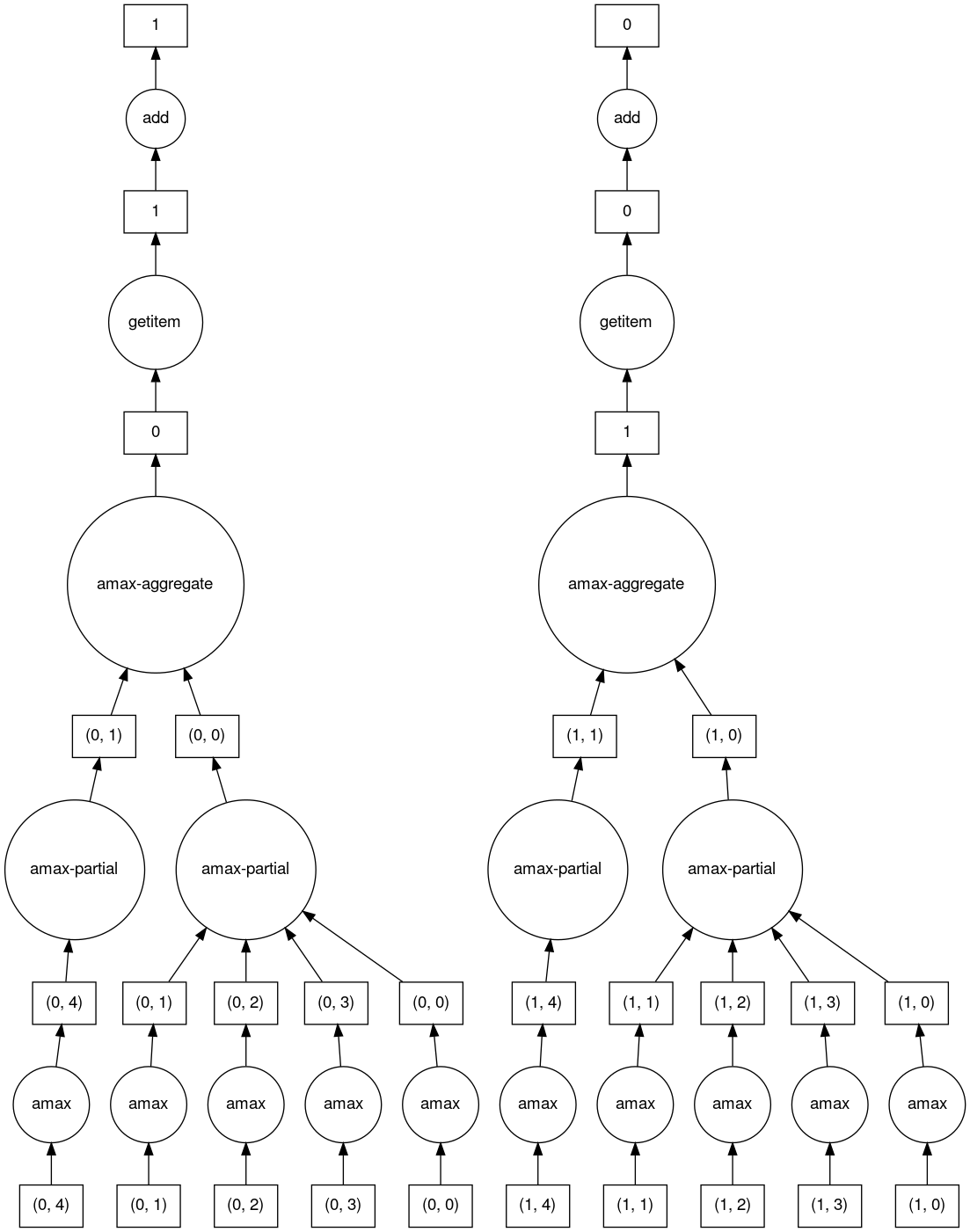
>>> b = a.max(axis=1)[::-1] + 10
... b
dask.array<add, shape=(200,), dtype=int64, chunksize=(100,), chunktype=numpy.ndarray>

>>> b[:10].compute()
array([100009,  99509,  99009,  98509,  98009,  97509,  97009,  96509,
      96009,  95509])
Dask Bag implements operations like map, filter, fold, and
groupby on collections of generic Python objects.
>>> b.filter(lambda x: x % 2)
dask.bag<filter-lambda, npartitions=2>

>>> b.filter(lambda x: x % 2).compute()
[1, 3, 5, 1]

>>> b.distinct()
dask.bag<distinct-aggregate, npartitions=1>

>>> b.distinct().compute()
[1, 2, 3, 4, 5, 6]
Methods can be chained together.
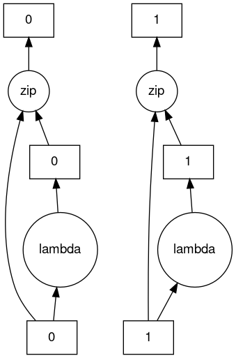
>>> c = db.zip(b, b.map(lambda x: x * 10))
... c
dask.bag<zip, npartitions=2>

>>> c.compute()
[(1, 10), (2, 20), (3, 30), (4, 40), (5, 50), (6, 60), (2, 20), (1, 10)]
Visualize the Task Graph#
So far we’ve been setting up computations and calling compute. In addition to
triggering computation, we can inspect the task graph to figure out what’s going on.
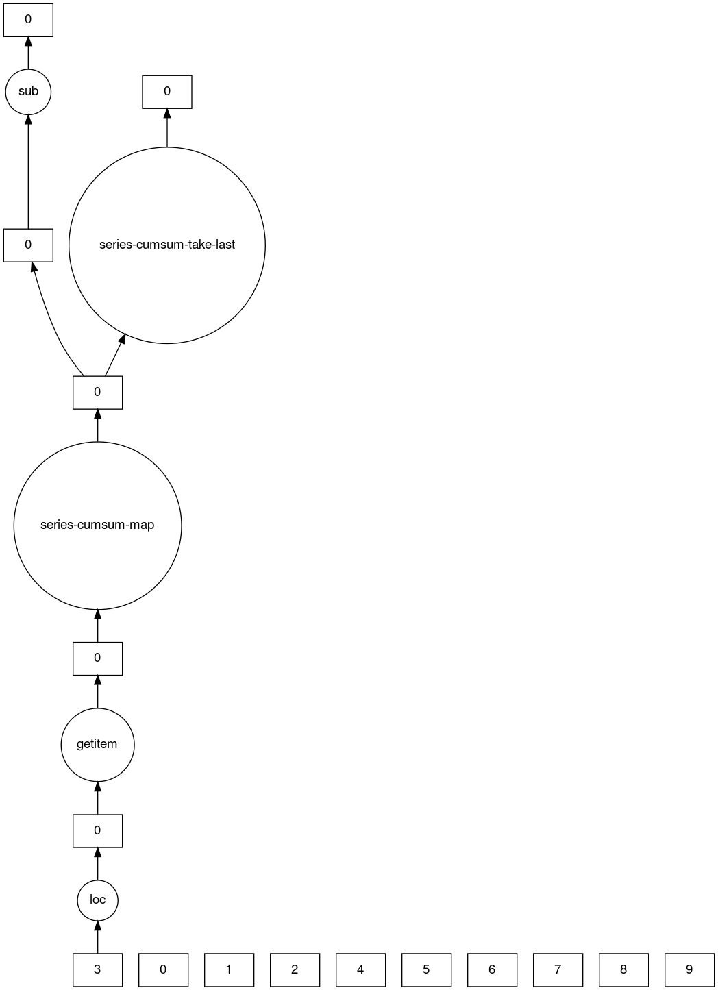
>>> result.dask
HighLevelGraph with 7 layers.
<dask.highlevelgraph.HighLevelGraph object at 0x7f129df7a9d0>
1. from_pandas-0b850a81e4dfe2d272df4dc718065116
2. loc-fb7ada1e5ba8f343678fdc54a36e9b3e
3. getitem-55d10498f88fc709e600e2c6054a0625
4. series-cumsum-map-131dc242aeba09a82fea94e5442f3da9
5. series-cumsum-take-last-9ebf1cce482a441d819d8199eac0f721
6. series-cumsum-d51d7003e20bd5d2f767cd554bdd5299
7. sub-fed3e4af52ad0bd9c3cc3bf800544f57

>>> result.visualize()
>>> b.dask
HighLevelGraph with 6 layers.
<dask.highlevelgraph.HighLevelGraph object at 0x7fd33a4aa400>
1. array-ef3148ecc2e8957c6abe629e08306680
2. amax-b9b637c165d9bf139f7b93458cd68ec3
3. amax-partial-aaf8028d4a4785f579b8d03ffc1ec615
4. amax-aggregate-07b2f92aee59691afaf1680569ee4a63
5. getitem-f9e225a2fd32b3d2f5681070d2c3d767
6. add-f54f3a929c7efca76a23d6c42cdbbe84

>>> b.visualize()
>>> c.dask
HighLevelGraph with 3 layers.
<dask.highlevelgraph.HighLevelGraph object at 0x7f96d0814fd0>
1. from_sequence-cca2a33ba6e12645a0c9bc0fd3fe6c88
2. lambda-93a7a982c4231fea874e07f71b4bcd7d
3. zip-474300792cc4f502f1c1f632d50e0272

>>> c.visualize()
Low-Level Interfaces#
Often when parallelizing existing code bases or building custom algorithms, you run into code that is parallelizable, but isn’t just a big DataFrame or array.
Dask Delayed lets you to wrap individual function calls into a lazily constructed task graph:
import dask

@dask.delayed
def inc(x):
   return x + 1

@dask.delayed
def add(x, y):
   return x + y

a = inc(1)       # no work has happened yet
b = inc(2)       # no work has happened yet
c = add(a, b)    # no work has happened yet

c = c.compute()  # This triggers all of the above computations
Unlike the interfaces described so far, Futures are eager. Computation starts as soon as the function is submitted (see Futures).
from dask.distributed import Client

client = Client()

def inc(x):
   return x + 1

def add(x, y):
   return x + y

a = client.submit(inc, 1)     # work starts immediately
b = client.submit(inc, 2)     # work starts immediately
c = client.submit(add, a, b)  # work starts immediately

c = c.result()                # block until work finishes, then gather result
Note
Futures can only be used with distributed cluster. See the section below for more information.
Scheduling#
After you have generated a task graph, it is the scheduler’s job to execute it (see Scheduling).
By default, for the majority of Dask APIs, when you call compute on a Dask object,
Dask uses the thread pool on your computer (a.k.a threaded scheduler) to run computations in parallel.
This is true for Dask Array, Dask DataFrame,
and Dask Delayed. The exception being Dask Bag
which uses the multiprocessing scheduler by default.
If you want more control, use the distributed scheduler instead. Despite having “distributed” in it’s name, the distributed scheduler works well on both single and multiple machines. Think of it as the “advanced scheduler”.
This is how you set up a cluster that uses only your own computer.
>>> from dask.distributed import Client
...
... client = Client()
... client
<Client: 'tcp://127.0.0.1:41703' processes=4 threads=12, memory=31.08 GiB>
This is how you connect to a cluster that is already running.
>>> from dask.distributed import Client
...
... client = Client("<url-of-scheduler>")
... client
<Client: 'tcp://127.0.0.1:41703' processes=4 threads=12, memory=31.08 GiB>
There are a variety of ways to set up a remote cluster. Refer to how to deploy dask clusters for more information.
Once you create a client, any computation will run on the cluster that it points to.
Diagnostics#
When using a distributed cluster, Dask provides a diagnostics dashboard where you can see your tasks as they are processed.
>>> client.dashboard_link
'http://127.0.0.1:8787/status'
To learn more about those graphs take a look at Dashboard Diagnostics.